Introduction

기존 open-vocabulary 3DGS segmentation 모델들을 panoptic segmentation task에 적용할 때의 문제점:

1. 부정확한 3D language feature learning
• 클래스별로 feature가 quantize된 경우 물체들끼리 의미적으로는 유사하더라도 language feature가 전혀 연관성 없게 학습될 수 있다.
• Feature compression을 수행하는 경우 feature의 성능이 약해질 수 있다.
2. Semantic 정보만 학습하지, instance 정보를 학습하지는 않는다.

이러한 한계점을 해결하기 위해, PanoGS는 우선 pyramid tri-plane 방식을 이용해 latent feature를 표현한다. 이를 통해 공간상에서 feature를 연속적으로 표현할 수 있다. 또한, PanoGS는 렌더링을 한 뒤 학습 signal을 생성하는 것이 아니라 fused feature cloud를 이용해 3D에서 직접 loss를 계산하기 때문에 alpha-blending으로 인한 error나 domain gap도 방지할 수 있다.

또한, instance 구분을 graph clustering problem으로 접근한다. 이를 통해 각 물체에 속한 가우시안을 일관된 클러스터로 묶을 수 있다.

Method

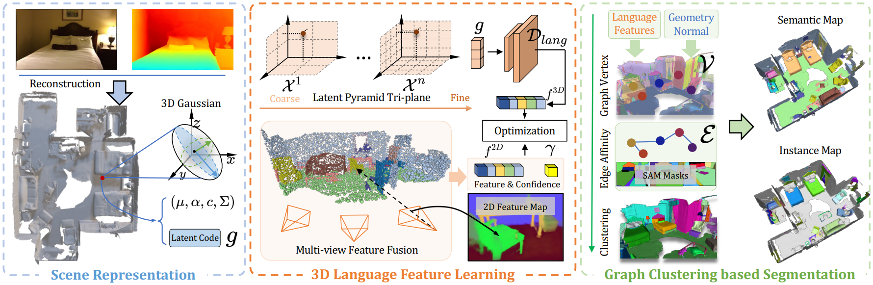
3D Language Feature Learning

Latent Pyramid Tri-plane

PanoGS는 RGBD 이미지를 입력으로 받아 3DGS를 우선 학습한다. 각 가우시안에 대해 latent language code $g$를 계산할 수 있는데, 이는 pyramid tri-plane을 통해 얻을 수 있다. 가우시안 중심점의 좌표가 $\mu$일 때, $g$를 구하는 식은 아래와 같다.

$g(\mu) = \sum\limits_{i}^{n} \{ \mathcal{T}(\mu, \mathcal{X}_{xy}^i), \mathcal{T}(\mu, \mathcal{X}_{yz}^i), \mathcal{T}(\mu, \mathcal{X}_{xz}^i) \}$

$\mathcal{T}(\cdot)$는 trilinear interpolation, $\mathcal{X}^i$는 $i$번째 pyramid 단계에서의 feature plane을 의미한다.

메모리 한계로 인해 $g(\mu)$의 dimension은 원래 language feature에 비해 매우 작다고 한다. 결국 feature compression이 일어나는 것이다. 따라서 이 저차원 feature code를 원래의 language feature로 복원하기 위해 decoder가 필요하다.

$f^{3D}(\mu) = \mathcal{D}_{lang}(g(\mu))$

Multi-view Feature Fusion

3D 가우시안을 특정 viewpoint로 렌더링할 수 있으므로 여러 view에서 렌더링된 RGB 이미지에 대해 LSeg feature를 구할 수 있다. 따라서 $i$번째 가우시안 1개에 대해 각 view에서의 2D feature vector $\{f_1, \cdots, f_m\}$를 얻을 수 있다. 이후 pooling operation $\Phi(\cdot)$을 이용해 그 가우시안에 대한 융합된 2D feature vector $f_i^{2D}(\mu)$를 얻는다.

이때 occlusion이나 multi-view inconsistency로 인해 각 view에서의 feature에 차이가 있을 수 있다. 따라서 각 view에 대한 $i$번째 가우시안의 confidence $\gamma_i^{2D}$도 함께 구한다.

$\gamma_i^{2D} = \cfrac{Obs(p_i)}{\sum_{D_l} Var(\{f_1, f_2, \cdots, f_m\})}$

$Obs(p_i)$는 $i$번째 가우시안이 valid하게 관측된 view의 개수를 의미하고, $Var(\cdot)$은 multi view language feature $\{f_1, \cdots, f_m\}$의 분산을 의미한다.

최종적으로, $N$개의 가우시안에 대한 2D fused feature $f_i^{2D}$와 confidence $\gamma_i^{2D}$를 얻을 수 있다. $(i = 1, \cdots, N)$

Language Feature Distillation

이제 $f^{3D}$와 $f^{2D}$의 비교를 통해 pyramid tri-plane과 decoder $\mathcal{D}_{lang}$을 학습한다. 구체적인 loss 함수는 cosine similarity loss로, 수식은 아래와 같다.

$\mathcal{L}_{feat} = \sum\limits_{i}^{N} \gamma_i^{2D} \cdot \left| 1 - \cos\left( \mathcal{D}_{lang}(g_i), f_i^{2D} \right) \right|$

Graph Clustering based Segmentation

PanoGS는 instance 정보 없이 우선 가우시안들을 클러스터링한다. 본 논문에서는 이 문제를 graph clustering task로 보고 scene graph $\mathcal{G} = (\{\mathcal{V}_i\}, \{\mathcal{E}_{ij}\})$를 만든다.

Graph Vertex Construction

각각의 가우시안을 노드로 보고 클러스터링하는 것은 매우 비효율적이기 때문에 물체보다는 작은 단위로 먼저 클러스터링을 진행한다. 이 방식을 language-guided graph cuts라 한다.

가우시안이 하나 이상 클러스터링된 것을 super-primitive라고 하는데, 두 super-primitive가 하나로 합쳐지는 경우는 둘의 normal vector의 cosine similarity가 특정 threshold 이상, 그리고 둘의 3D language feature의 cosine similarity가 특정 threshold 이상일 때이다.

이를 통해 geometry 정보와 semantic 정보가 일관된 작은 클러스터들을 생성하였다. 이러한 클러스터들은 graph $\mathcal{G}$의 노드 $\mathcal{V}_i$가 된다.

Edge Affinity Computation

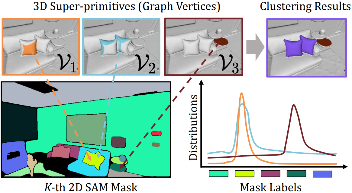
노드를 생성한 후에는 노드간 실제 거리를 이용하여 affinity를 계산한다. 이를 위해 SAM mask를 사용한다. Affinity를 얻기 위해, 우선 두 super primitives $\mathcal{V}_i, \mathcal{V}_j$를 2D로 렌더링한다. 이후 각 가우시안은 그 primitive가 속한 SAM mask의 index를 갖는다. 두 super primitives가 같은 SAM mask로 렌더링되었다면 각각의 가우시안은 대부분 같은 index를 가질 것이다.

위 그림의 그래프는 각 super primitive에 속한 가우시안들이 어떤 SAM mask index를 가지는지를 distribution으로 나타낸 것이다. 이 distribution이 유사한 두 super primitive들은 affinity가 크다고 볼 수 있다. Distribution의 유사도는 Jensen-Shannon divergence를 이용해 계산한다.

이러한 연산을 multi-view에서 수행하여 noise를 줄인다. 각 view에서의 affinity를 산술평균하여 최종 affinity $\mathcal{E}_{ij}$를 구한다.

Progressive Graph Clustering

$\mathcal{G} = (\{\mathcal{V}_i\}, \{\mathcal{E}_{ij}\})$를 구했으므로 이를 이용해 최종 클러스터링을 진행한다. 총 4번의 iteration을 진행하는데, 0.9부터 0.6까지 threshold를 낮춰 가며 그 값보다 높은 affinity를 가지는 두 노드를 병합한다.

Open Vocabulary Panoptic Segmentation

Feature decoder를 이용해 각각의 가우시안에 대한 3D language feature를 구할 수 있다. 따라서 가장 많은 가우시안 feature에 해당하는 lauguage label을 그 instance의 label로 본다.

Experiments

Experimental Settings

데이터셋으로는 Replica와 ScanNetV2를 사용하였다. Metric으로는 mIoU, mAcc, 3D Panoptic Reconstruction Quality (PRQ)를 사용하였다. 특히, PRQ (T)는 things에 대한 metric, PRQ (S)는 stuff에 대한 metric으로 구분하였다.

Main Experiments

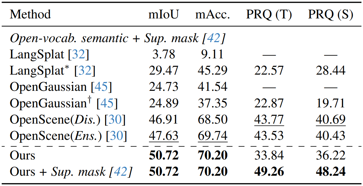
ScanNetV2에서의 실험 결과는 위 표와 같다.

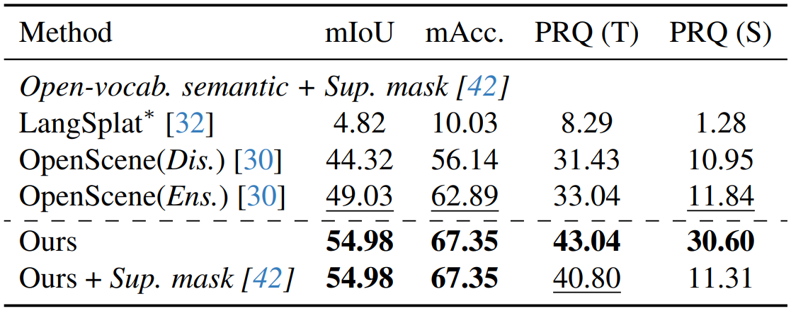
Replica에서의 실험 결과는 위 표와 같다.

PanoGS는 3D 공간에서 연속적인 language feature를 학습하기 때문에 더 좋은 성능이 나온 것으로 분석하고 있다.

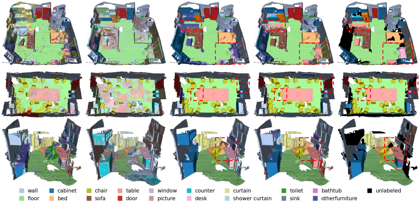
Semantic segmentation 결과를 시각화하면 위와 같다.

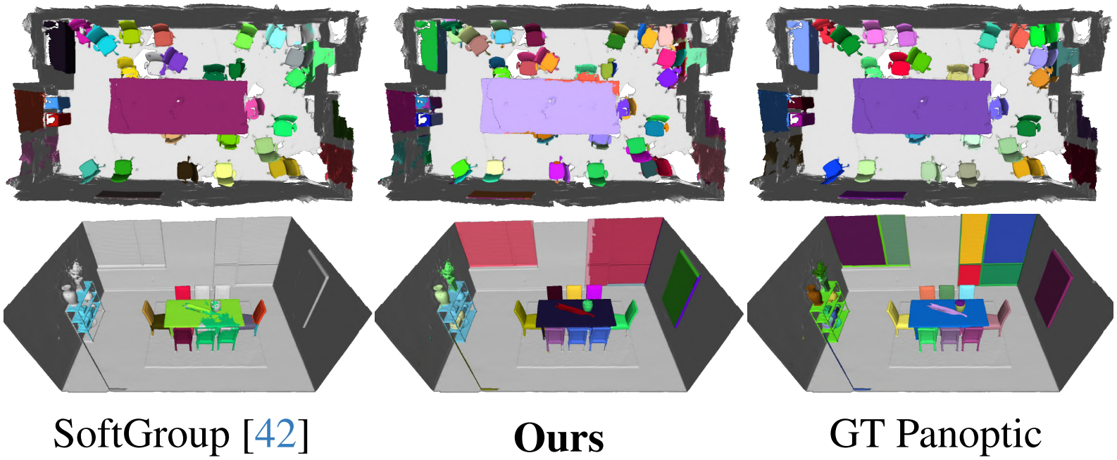
Panoptic segmentation 결과를 시각화하면 위와 같다.

Ablation Studies and Analysis

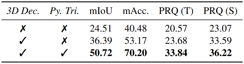
3D language feature learning에 관한 ablation study 결과는 위와 같다. 3D decoder와 pyramid tri-plane의 영향을 볼 수 있다.

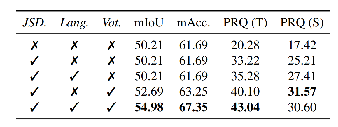
Graph clustering 관련 ablation study 결과는 위와 같다. Multi-view JSD를 사용했을 때, language-guided graph cuts를 사용했을 때, voting 과정을 사용했을 때의 영향을 각각 실험하였다. JSD를 사용하지 않은 경우는 단순 feature간 cosine similarity를 사용하였다.

Conclusion

PanoGS는 3DGS 기반으로 3D panoptic segmentation을 하는 모델이다. Latent pyramid tri-plane을 이용하여 3D language feature를 학습하였고, launguage-guided graph cuts를 통해 instance끼리도 분리하였다.