Introduction

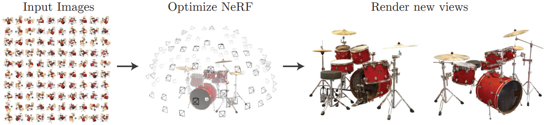
Neural Radiance Fields (NeRF) is a new method for synthesizing novel views of complex scenes. NeRF represents a static scene as a single MLP that outputs the volume density and view-dependent emitted radiance at any 3D point and viewing direction. The system uses classic volume rendering techniques to project the output colors and densities into an image. Since volume rendering is naturally differentiable, the entire system can be trained end-to-end with a set of images with known camera poses. The authors effectively optimized neural radiance fields to render photorealistic novel views of scenes with complicated geometry and appearance.

The main contributions of this system are:

• An approach for representing continuous scenes as 5D neural radiance fields, parameterized as basic MLP networks.
• A differentiable rendering procedure based on classical volume rendering techniques, which is used to optimize NeRF from standard RGB images.
• A hierarchical sampling strategy to allocate the MLP's capacity towards space with visible scene content.
• A positional encoding to optimize NeRF to represent high-frequency scene content.

Related Work

Recent direction of view synthesis is to encode objects and scenes into the weights of an MLP, which directly produces 3D implicit representation of the shape. However, these methods are unable to reproduce the same fidelity as explicit methods such as meshes or voxel grids.

Neural 3D shape representations

Recent methods uses deep networks that directly generates continuous 3D shapes, such as Signed Distance Functions (SDFs) or occupancy fields. The downside of these methods is that they require ground truth 3D geometry for training, which is difficult to obtain for real-world scenes. Subsequent works have proposed to train these networks from 2D images. Still, these methods have so far been limited to simple shapes with low geometric complexity, resulting in oversmoothed renderings.

View synthesis and image-based rendering

A lot of works have been done on novel view synthesis with sparser view sampling. One popular family of approaches uses mesh-based representations. Predicted meshes are rasterized into 2D images, which are then compared with the ground truth 2D images to train the model by gradient descent. However, gradient descent on meshes is often difficult and requires a template mesh with fixed topology, which is typically not available for real-world scenes.

Another class of methods use voxel grids. They are able to realistically represent complex shapes and materials, are well-suited for gradient-based optimization, and tend to produce less visually distracting artifacts than mesh-based methods. Large datasets of scenes are used to train deep networks that predict a sampled volumetric representation, and novel views are rendered by using either alpha-compositing or learned compositing along rays. However, these methods requires a large amount of computation and memory due to their explicit nature.

NeRF is a continuous representation that does not suffer from computation and memory limitations. NeRF produces significantly higher quality renderings than prior volumetric approaches, with just a fraction of the storage cost of those sampled volumetric representations.

Neural Radiance Field Scene Representation

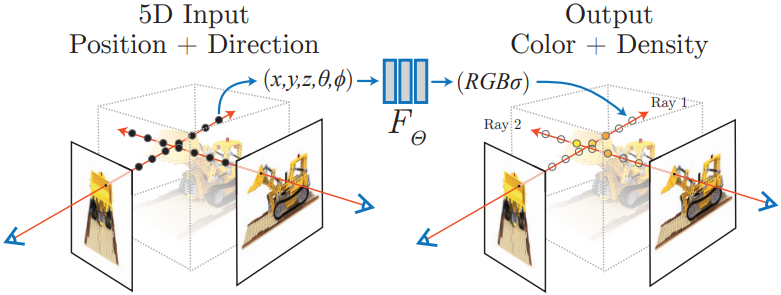
The scene is represented as a function whose input is a 3D location $\mathbf{x} = (x, y, z)$ and 2D viewing direction $\mathbf{d} = (\theta, \phi)$, and whose output is an emitted color $\mathbf{c} = (r, g, b)$ and volume density $\sigma$.

A single MLP is used to represent the entire scene. The network takes $(\mathbf{x}, \mathbf{d})$ as input and outputs $(\mathbf{c}, \sigma)$. The network predicts the volume density $\sigma$ as a function of only the location $\mathbf{x}$, while allowing the RGB color $\mathbf{c}$ to be predicted as a function of both location and viewing direction.

To accomplish this, the MLP first processes the input 3D coordinate $\mathbf{x}$ with 8 fully-connected layers, and outputs $\sigma$ and a 256-dimensional feature vector. This feature vector is then concatenated with the camera ray's viewing direction $\mathbf{d}$ and passed to one additional fully-connected layer that outputs the view-dependent RGB color $\mathbf{c}$.

Volume Rendering with Radiance Fields

Volume rendering means integrating the radiance along the viewing ray to produce the final pixel value. Radiance is the amount of light that passes through a surface in a given direction, and the radiance of a point is obtained from the output of the MLP. Viewing ray is a ray that starts at the camera center and passes through a pixel in the image plane.

Formally, the expected pixel color $C(\mathbf{r})$ of camera ray $\mathbf{r} = (\mathbf{o} + t\mathbf{d})$ with near and far bounds $t_n$ and $t_f$ is:

$C(\mathbf{r}) = \int_{t_n}^{t_f}T(t)\sigma(\mathbf{r}(t))\mathbf{c}(\mathbf{r}(t), \mathbf{d})dt$

where

$T(t) = \exp\left(-\int_{t_n}^{t}\sigma(\mathbf{r}(t'))dt'\right).$

The function $T(t)$ is the transmittance, which is a probability that the ray travels from $t_n$ to $t$ without hitting any other particle.

$\sigma(\mathbf{r}(t))$ is a probability that the ray hits a particle at $\mathbf{r}(t)$, and $\mathbf{c}(\mathbf{r}(t), \mathbf{d})$ is the RGB color emitted by the particle at $\mathbf{r}(t)$ in the direction $\mathbf{d}$.

To implement this continuous integral in practice, the system uses a stratified sampling approach where $[t_n, t_f]$ is partitioned into $N$ evenly-spaced bins and then draw one sample uniformly at random from within each bin.

This stratified sampling enables a continuous scene representation because it results in the MLP being evaluated at continuous positions over the course of optimization.

Optimizing a Neural Radiance Field

Before getting into the loss function, two important strategies are used: positional encoding and hierarchical volume sampling.

Positional Encoding

Since deep networks are biased towards learning lower frequency functions, mapping the inputs to a higher dimensional space using high frequency functions before passing them to the network enables better fitting of data that contains high frequency variation. Having the network directly operate on the input results in poor representation of high-frequency variation in color and geometry.

The paper introduces a positional encoding function $\gamma(p)$ that maps a coordinate value $p$ to a higher dimension space $\mathbb{R}^{2L}$:

$\gamma(p) = \left[\sin(2^0p), \cos(2^0p), \sin(2^1p), \cos(2^1p), \ldots, \sin(2^{L-1}p), \cos(2^{L-1}p)\right]$

This function is applied separately to both coordinate and viewing direction inputs, which are normalized beforehand. Then the output of the positional encoding is concatenated with the input before passing it to the network. The authors used $L = 10$ for $\gamma(\mathbf{x})$ and $L = 4$ for $\gamma(\mathbf{d})$.

Hierarchical Volume Sampling

The stratified sampling approach is used to sample the radiance along the viewing ray. However, this approach is inefficient in that points in free space and occluded region are still sampled repeatedly.

Instead of using only one MLP to represent the entire scene, they use two MLPs together to represent the scene: one coarse, one fine. They first run the coarse network on a set of $N_c$ locations using stratified sampling to produce a more informed sampling of points along each ray. These samples are biased towards the relevant parts of the volume. $N_f$ additional samples are then drawn from the relevant parts of the volume based on the result of the coarse network. The fine network is then ran on all $N_c + N_f$ samples to produce the final output.

Optimization and Loss Function

Optimization requires a dataset of captured RGB images of the scene, the corresponding camera poses and intrinsic parameters, and scene bounds. At each optimization iteration, a batch of camera rays are randomly sampled from the set of all pixels in the dataset. Then the points are sampled along the camera rays following the hierarchical sampling strategy above; $N_c$ points for the coarse network and $N_c + N_f$ points for the fine network. The volume rendering procedure is used to render the color of each ray from both sets of samples.

The loss is simply the total squared error between the rendered and true pixel colors for both the coarse and fine renderings:

$L = \sum_{\mathbf{r}\in\mathcal{R}} \left[ ||\hat{C}_c(\mathbf{r}) - C(\mathbf{r})||_2^2 + ||\hat{C}_f(\mathbf{r}) - C(\mathbf{r})||_2^2 \right]$

where $\hat{C}_c(\mathbf{r})$ and $\hat{C}_f(\mathbf{r})$ are the colors predicted by the coarse and fine networks, respectively, and $C(\mathbf{r})$ is the true pixel color. Even though the final rendering comes from $\hat{C}_f(\mathbf{r})$, the loss of $\hat{C}_c(\mathbf{r})$ is also minimized so that the weight distribution from the coarse network can be used to allocate samples in the fine network.

Results

Datasets

DeepVoxels dataset is used for synthetic renderings, and LLFF dataset is used for real-world scenes. They also generated their own datasets for both synthetic and real-world scenes.

Baselines

Neural Volumes (NV), Scene Representation Networks (SRNs), and Local Light Field Fusion (LLFF) are used as baselines.

Quantitative Results

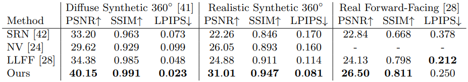
NeRF quantitatively outperforms prior work on datasets of both synthetic and real images.

Qualitative Results

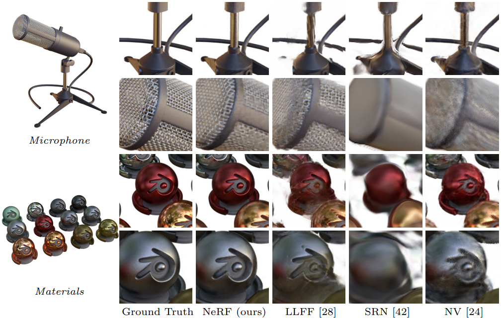
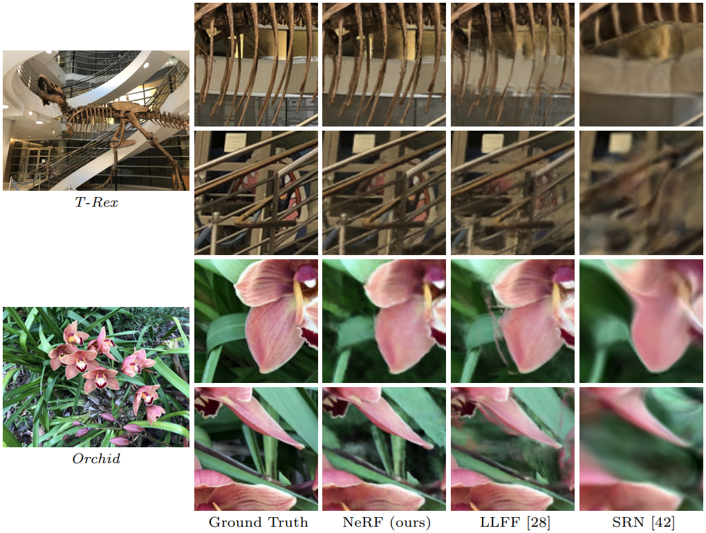
NeRF achieves better multiview consistency and produces fewer artifacts than all baselines, in both synthetic and real-world scenes. NeRF is able to represent fine geometry more consistently across rendered views. NeRF also correctly reconstructs partially occluded regions that LLFF struggles to render cleanly.

Ablation Studies

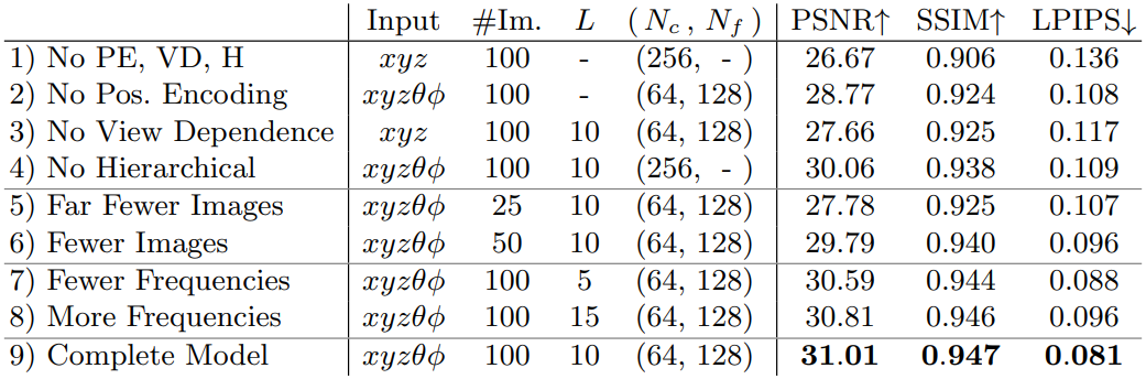
Positional encoding (row 2) and view-dependence (row 3) provide the largest quantitative benefit followed by hierarchical sampling (row 4). Rows 5-6 show how the performance decreases as the number of input images is reduced. Rows 7-8 validates the choice of the frequency used in the positional encoding.

Conclusion

Representing scenes as 5D neural radiance fields produces better renderings than the previously-dominant approaches. However, there is still much more progress to be made in efficiently optimizing and rendering neural radiance fields. Another direction for future work is interpretability: explicit representations such as voxel grids and meshes admit reasoning about the expected quality of rendered views and failure modes, but it is unclear how to analyze these issues when the scenes are encoded in the weights of a deep neural network.