To Begin With

This is a summary of the second part of the ICP & Point Cloud Registration series by Prof. Cyrill Stachniss. Lecture slides and videos are available on the course website or his YouTube channel. Through this series, we will learn the basics of the Iterative Closest Point (ICP) algorithm and build the code from scratch.

We Can't Always Find the 'Right' Correspondences

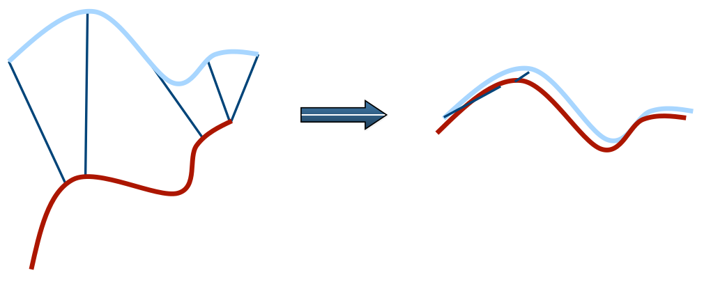
In the previous post, we assumed that we know the 'perfect' correspondences between two point clouds. However, in practice, we cannot find the correct correspondences. With imperfect correspondences, it is generally impossible to determine the optimal parameters in one step.

Since we do not know the correspondences, we need to identify the most probable pair of points that is from the same spot of the object/environment. The most simple and intuitive way to do this is to match the closest point for each point in the source point cloud. The resulting parameters, $\mathbf{R}$ and $\mathbf{t}$, will not be perfect, but will bring the source point cloud closer to the target point cloud than before. By iterating this process, we can gradually improve the parameters and the correspondences. This is the basic idea of the ICP algorithm. The following figure shows the process of the ICP algorithm with the closest point matching.

Outline of the Algorithm

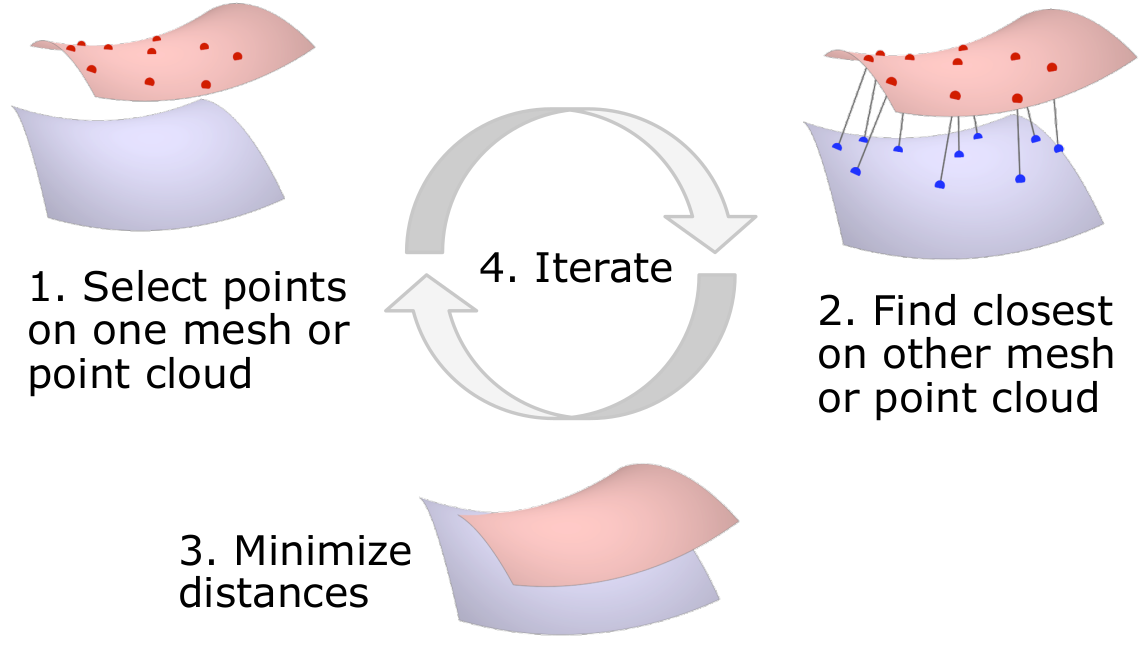
The ICP algorithm is an iterative algorithm that repeats the following steps until the algorithm converges.

1. Make an initial guess for the parameters $\mathbf{R}$ and $\mathbf{t}$.
2. Find the closest point for each point in the source point cloud and compute $\mathbf{R}$ and $\mathbf{t}$.
3. Transform the source point cloud with the optimal parameters.
4. Repeat steps 2-3 until the algorithm converges.

The algorithm converges when the difference between the previous and current parameters is smaller than a certain threshold.

The pseudo code of the ICP algorithm is as follows.

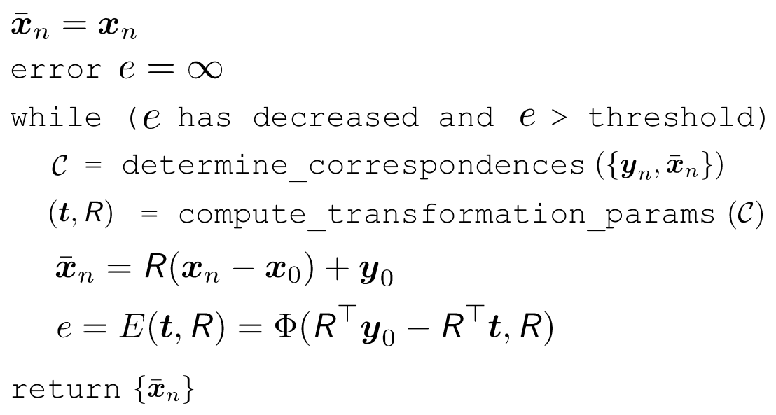
$x_n$ and $y_n$ are the source and target point clouds, respectively. At line 1, we make an initial guess. $\bar{x_n}$ is the transformed source point cloud. Initially, $\bar{x_n}$ is the same as $x_n$. At line 2, we set an error term as infinity. The error term is the difference between the previous and current parameters. We will take a deeper look at the error term later. At line 3, we iterate the following steps until the error term is smaller than a certain threshold. At line 4, we find the closest point for each point in the source point cloud. At line 5, we compute the optimal parameters. At line 6, we transform the source point cloud with the optimal parameters. At line 7, we compute the error term. At line 8, we return the updated source point cloud.

ICP Variants

Some steps of ICP can be modified to improve the performance. In my opinion, these modification strategies are the most important part of the ICP algorithm. In practice, the following modifications are widely used.

1. Consider point subsets: Increase speed
2. Different data association strategies: Increase stability
3. Weight the correspondences: Increase tolerance w.r.t. noise and outliers
4. Reject potential outlier point pairs: Increase the basin of convergence

1. Consider Point Subsets

In practice, the point clouds are usually too large to be processed at once. We can consider point subsets instead of the entire point clouds. There are multiple ways to select point subsets.

• Uniform sampling
• Normal-space sampling
• Feature-based sampling
• Random sampling

The following figure illustrates the difference between uniform and normal-space sampling.

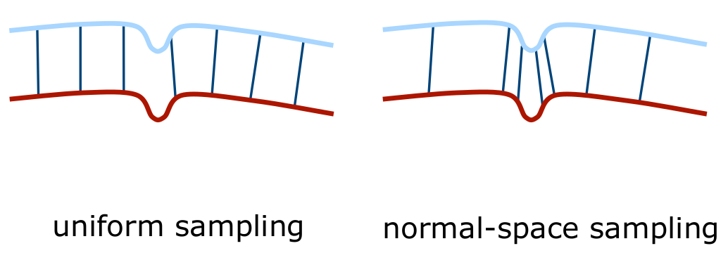
In uniform sampling, we select points uniformly throughout the entire space. That is, we select less points from the dense area and more points from the sparse area. On the other hand, in normal-space sampling, we select points from the point cloud based on the normal vectors, so that the direction of the normal vectors is uniform. Therefore, the normal-space sampling is more robust to noise and outliers.

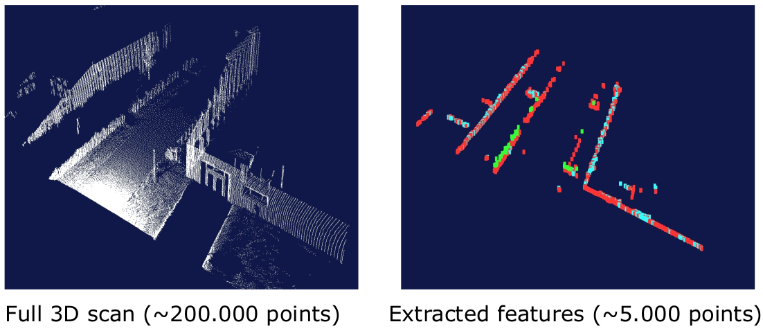
Moreover, when we can extract reliable features from the point clouds, we can use the features to select point subsets. For example, we can select points from the feature points or points near the feature points. This method may result in higher accuracy and faster convergence with less number of points, depending on how accurate the features are.

2. Different Data Association Strategies

As mentioned earlier, the closest point matching is the most simple and intuitive way to find the correspondences. However, it is not always the best way. In practice, we can use different data association strategies to find the correspondences.

• Closest compatible point
• Normal shooting
• Projection-based approaches
• Point-to-plane
• ...

Closest compatible point is a simple extension of the closest point matching. We can use more constraints about the correspondences, e.g., color of the point when the camera is accessable.

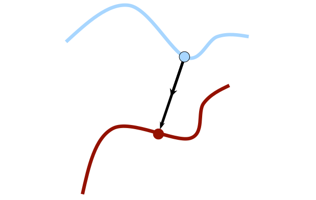
Normal shooting is a method that uses the normal vectors of the points. From each point in the source point cloud, we shoot a ray in the direction of the normal vector. Then, we find the closest point that the ray hits in the target point cloud. The following figure illustrates the normal shooting method.

Normal shooting shows slightly better convergence results than closest point for smooth structures, but worse for noisy or complex structures.

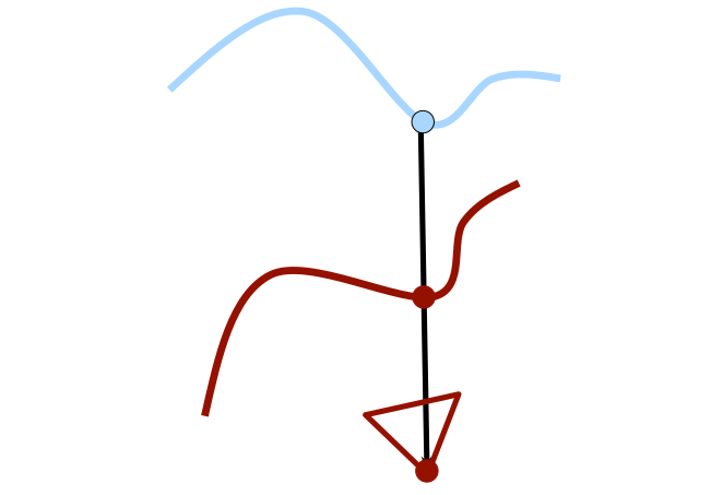
Projection-based approaches are similar to normal shooting, but shoots a ray in the direction from the sensor to the point, and choose the closest point that the ray hits.

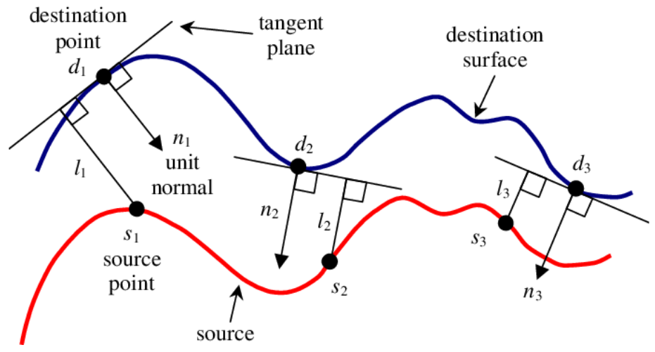
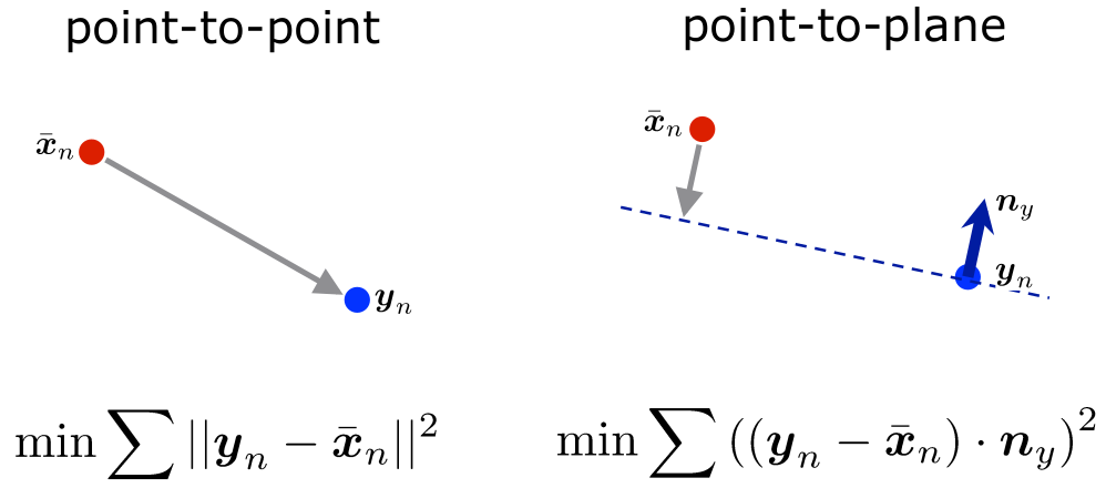
Point-to-plane is a most widely used method in practice. It calculates the distance from the point to the plane by adding only one more calculation. As you can see in the figure above, the point-to-point distance is dot producted with the normal vector of the plane, resulting in the point-to-plane distance. This method generally shows better convergence results than point-to-point method.

3. Weight the Correspondences

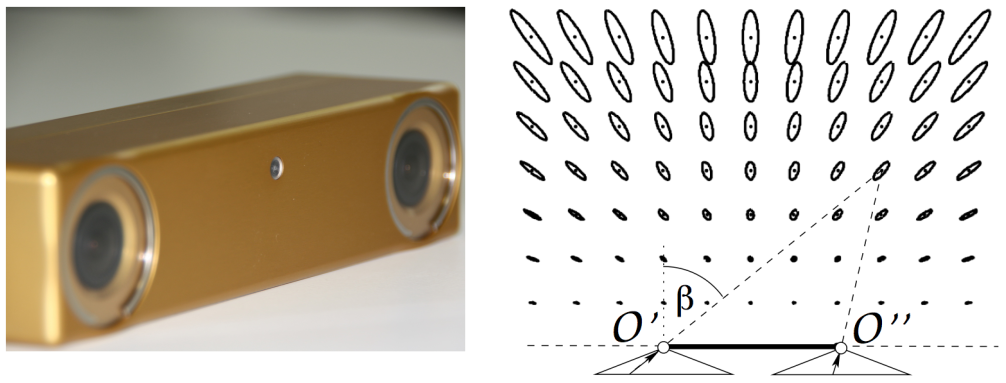
In practice, the point clouds are usually noisy and contain outliers. Therefore, we can weight the correspondences to increase the tolerance w.r.t. noise and outliers. Especially, we can deal with sensor noises which are generally larger as the distance from the sensor increases, by applying less weight to the further points. The following figure illustrates the conceptual idea of this noise.

4. Reject Potential Outlier Point Pairs

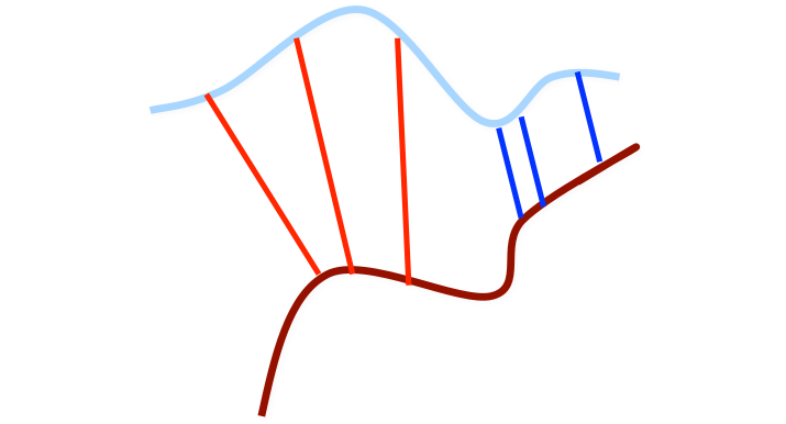
In practice, the point clouds may contain outliers. To be simple, we can ignore the pairs of points with larger distances than a certain threshold. The following figure illustrates this method.

In a Nutshell

We learned the basic idea of the ICP algorithm and its variants. Let's sum up all the steps needed to implement the ICP algorithm.

1. Downsample source point cloud.
2. Find the correspondences using the appropriate method mentioned above.
3. Optionally weight the correspondences or reject potential outlier point pairs.
4. Compute the optimal parameters $\mathbf{R}$ and $\mathbf{t}$ using SVD.
5. Transform the source point cloud with the optimal parameters.
6. Compute the error term.
7. Repeat steps 2-6 until the algorithm converges.

In the next post, we will implement the most basic ICP algorithm using ROS1 and C++. Stay tuned!