To Begin With

This is a summary of the first part of the ICP & Point Cloud Registration series by Prof. Cyrill Stachniss. Lecture slides and videos are available on the course website or his YouTube channel. Through this series, we will learn the basics of the Iterative Closest Point (ICP) algorithm and build the code from scratch.

What is ICP?

Iterative Closest Point (ICP) is an algorithm to register two point clouds. Point cloud is a set of points in 3D space, and registration is a process of aligning two point clouds. What this algorithm does is better explained with a picture.

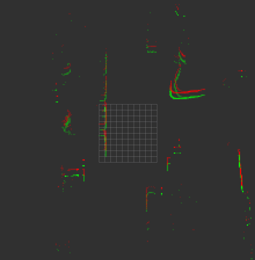
The red markers indicate the first 2D Lidar scan and the green markers indicate the second. Imagine we are in a self-driving car, and the Lidar sensor is scanning the environment. Intuitively, we understand that the car is moving forward because the dots appear to be moving backward. But here is the question for the car: Where exactly is the car located, and how far has it actually moved? These are fundamental question in the field of self-driving car and mobile robotics, since precise localization is tightly related with safety, efficiency, and accuracy.

Overview

ICP is a simple and strong algorithm for estimating the transformation between the two point clouds, which can be directly used to derive the past trajectory of the car or robot. The algorithm is as follows:

1. Find the closest point in the second point cloud for each point in the first point cloud.
2. Compute the transformation that aligns the first point cloud to the second point cloud.
3. Apply the transformation to the first point cloud.
4. Repeat 1-3 until convergence.

Through this series of posts, we will go through each step in detail. In this post, we will focus on computing the transformation given the perfectly matching pairs of points (correspondences).

Key Terms and Parameters

Before we dive into the algorithm, let's define some key terms and parameters that will be used throughout this series. We will use the following notations:

Key Terms

• Correspondence: A pair of points that are known to be the same. For the sake of simplicity, we artificially designate two points as corresponding if they share the same index, $i$. $x_i$ and $y_i$ are the same point in different point cloud.
• Registration: The process of finding the rotation matrix $\mathbf{R}$ and translation vector $\mathbf{t}$ that aligns the two point clouds $\mathbf{X}$ and $\mathbf{Y}$.

Parameters

• Reference (first) point cloud: $\mathbf{Y} = \{y_1, y_2, \cdots, y_n\}$
• Incoming (second) point cloud: $\mathbf{X} = \{x_1, x_2, \cdots, x_n\}$
• Rotation matrix and translation vector: $\mathbf{R}$ and $\mathbf{t}$
• Transformed point cloud: $\bar{\mathbf{X}} = \{\bar{x}_1, \bar{x}_2, \cdots, \bar{x}_n\}$

Therefore, our dataset is defined as described above, consisting of corresponding points such as x1 and y1, x2 and y2, etc., which represent the same point observed from different locations. Note that the coordinate system used is x-forward and y-left.

One-Shot Optimal Solution

As mentioned earlier, it has been proven that a one-shot direct algorithm exists for registering two point clouds, provided the correct correspondences are known. The core technique utilized in this process is Singular Value Decomposition (SVD). The procedure involves several key steps:

1. Determine the centroid for each point cloud.
2. Shift both point clouds such that their centroids coincide with the origin.
3. Construct the rotation matrix $\mathbf{R}$ that aligns the two point clouds.
4. Shift both point clouds back to their initial positions and rotate the second point cloud by $\mathbf{R}$.
5. Find the translation vector $\mathbf{t}$ that aligns the two point clouds.

Quite simple, isn't it? This direct method can be done only if the correct correspondences are known, which means that we know the first point cloud and the second point cloud are the same point observed from different locations. In the next section, we will derive the mathematical formulation for each step.

1. Determine the centroid for each point cloud.

The centroid of a point cloud is the average of all points in the point cloud. It can be computed as follows:

$x_0 = \frac{1}{n} \sum_{i=1}^{n} x_i$

$y_0 = \frac{1}{n} \sum_{i=1}^{n} y_i$

2. Shift both point clouds such that their centroids coincide with the origin.

The centroid of each point cloud is subtracted from all points in the point cloud. This operation shifts the centroid to the origin.

$x_i = x_i - x_0$

$y_i = y_i - y_0$

3. Construct the rotation matrix $\mathbf{R}$ that aligns the two point clouds.

3.1. Compute the covariance matrix $\mathbf{H}$ of the two point clouds $\mathbf{X}$ and $\mathbf{Y}$.

The covariance matrix $\mathbf{H}$ is a square matrix that contains the covariance between each pair of elements of a vector. The covariance between two elements $x_i$ and $y_i$ is computed as follows:

$cov(x_i, y_i) = \sum_{i=1}^{n} (x_i - x_0)(y_i - y_0)$

The covariance matrix $\mathbf{H}$ is computed as follows:

$\mathbf{H} = \sum_{i=1}^{n} (x_i - x_0)(y_i - y_0)$

3.2. Construct the rotation matrix $\mathbf{R}$.

The rotation matrix $\mathbf{R}$ is constructed using Singular Value Decomposition (SVD). SVD is a technique to decompose a matrix into three matrices, as follows:

$\mathbf{H} = \mathbf{U} \mathbf{D} \mathbf{V}^T$

$\mathbf{U}$ and $\mathbf{V}$ are orthogonal matrices, and $\mathbf{D}$ is a diagonal matrix. The diagonal elements of $\mathbf{D}$ are called singular values. The singular values are sorted in descending order. The first column of $\mathbf{U}$ is called the left singular vector, and the first column of $\mathbf{V}$ is called the right singular vector. The left singular vector and the right singular vector are orthogonal to each other. The left singular vector and the right singular vector corresponding to the largest singular value are called the principal components. The principal components are the directions of the largest variance of the data. The principal components are also called the principal axes.

The rotation matrix $\mathbf{R}$ is constructed using the principal components of $\mathbf{X}$ and $\mathbf{Y}$ as follows:

$\mathbf{R} = \mathbf{V} \mathbf{U}^T$

4. Shift both point clouds back to their initial positions and rotate the second point cloud by $\mathbf{R}$.

The rotation matrix $\mathbf{R}$ is applied to the second point cloud $\mathbf{X}$ as follows:

$\bar{x}_i = \mathbf{R} x_i$

5. Find the translation vector $\mathbf{t}$ that aligns the two point clouds.

The translation vector $\mathbf{t}$ is computed as follows. The translation vector $\mathbf{t}$ is the difference between the centroid of the second point cloud $\mathbf{X}$ and the centroid of the rotated second point cloud $\bar{\mathbf{X}}$.

$\mathbf{t} = \frac{1}{n} \sum_{i=1}^{n} (\bar{x}_i - x_i) = \frac{1}{n} \sum_{i=1}^{n} (\mathbf{R} x_i - x_i)$