NICE
Flow model의 transformation 함수 $\mathbf{f}_{\theta}$는 모델마다 차이가 있는데, 가장 간단한 모델인 NICE부터 알아보자. NICE에서 각각의 transformation layer를 additive coupling layer라고 한다.
우선 latent vector $\mathbf{z}$를 두 그룹으로 쪼갠다. 첫 그룹 $\mathbf{z}_{1:d}$는 첫 $d$개의 element를, 두 번째 그룹 $\mathbf{z}_{d+1:n}$은 나머지 $n - d$개의 element를 가지고 있다. 각 layer에서 두 그룹에 속하는 element들은 각각 다르다.
Forward mapping $\mathbf{z} \mapsto \mathbf{x}$는 아래와 같이 정의된다.
$\begin{gather} \mathbf{x}_{1:d} = \mathbf{z}_{1:d} \\ \mathbf{x}_{d+1:n} = \mathbf{z}_{d+1:n} + m_{\theta}(\mathbf{z}_{1:d}) \end{gather}$
우선 첫 그룹 $\mathbf{z}_{1:d}$는 아무 변환 없이 그대로 $\mathbf{x}_{1:d}$가 된다. 두 번째 그룹에서는 $m_{\theta}(\mathbf{z}_{1:d})$를 더해주게 되는데, $m_{\theta}$는 input dimension $d$, output dimension $n - d$인 뉴럴 네트워크이다. 각 layer에서 $m_{\theta}$의 파라미터 $\theta$는 모두 다르다.
Inverse mapping $\mathbf{x} \mapsto \mathbf{z}$는 아래와 같다.
$\begin{gather} \mathbf{z}_{1:d} = \mathbf{x}_{1:d} \\ \mathbf{z}_{d+1:n} = \mathbf{x}_{d+1:n} - m_{\theta}(\mathbf{x}_{1:d}) \end{gather}$
첫 그룹은 아무 변환 없이 그대로 대입하면 되고, 두 번째 그룹은 단순히 $m_{\theta}$ 항을 좌변으로 넘겨주면 된다. 이때 $m_{\theta}$의 파라미터 $\mathbf{z}_{1:d}$가 $\mathbf{x}_{1:d}$와 동일하므로 파라미터도 그대로 쓸 수 있다.
Forward mapping에 대한 jacobian은 아래와 같이 구할 수 있다.
$J = \cfrac{\partial \mathbf{x}}{\partial \mathbf{z}} = \begin{pmatrix} I_d & 0 \\ \cfrac{\partial \mathbf{x}_{d+1:n}}{\partial \mathbf{z}_{1:d}} & I_{n-d} \end{pmatrix}$
대각 성분들은 모두 identity matrix인데, $\mathbf{x}$와 $\mathbf{z}$ 사이에 scaling이나 nonlinearity 없이 shift만 이루어지고 있기 때문이다. 또한 $\mathbf{x}_{1:d}$는 $\mathbf{z}_{d+1:n}$의 영향을 받지 않기 때문에 upper trangular 성분들은 모두 $0$이다.
Triangular matrix의 determinant는 대각 성분의 곱이기 때문에 위 jacobian matrix의 determinant는 $1$이다. 이로 인해 volume preserving transformation이라고도 불린다.
NICE에서는 이러한 additive coupling layer를 여러 층으로 쌓고, 마지막 layer로 rescaling layer를 추가한다. 이는 아래와 같이 정의된다.
$x_i = s_i z_i$
즉, 단순히 $\mathbf{z}$를 element-wise scaling하여 최종 $\mathbf{x}$를 구하는 것이다. 이때 $s_i$는 learnable parameter다.
이 rescaling layer에 대한 inverse mapping 또한 아래와 같이 간단하게 표현된다.
$z_i = \cfrac{x_i}{s_i}$
Jacobian matrix는 $J = \text{diag}(\mathbf{s})$이므로 determinant는 $\det(J) = \prod\limits_{i=1}^{n} s_i$가 된다.
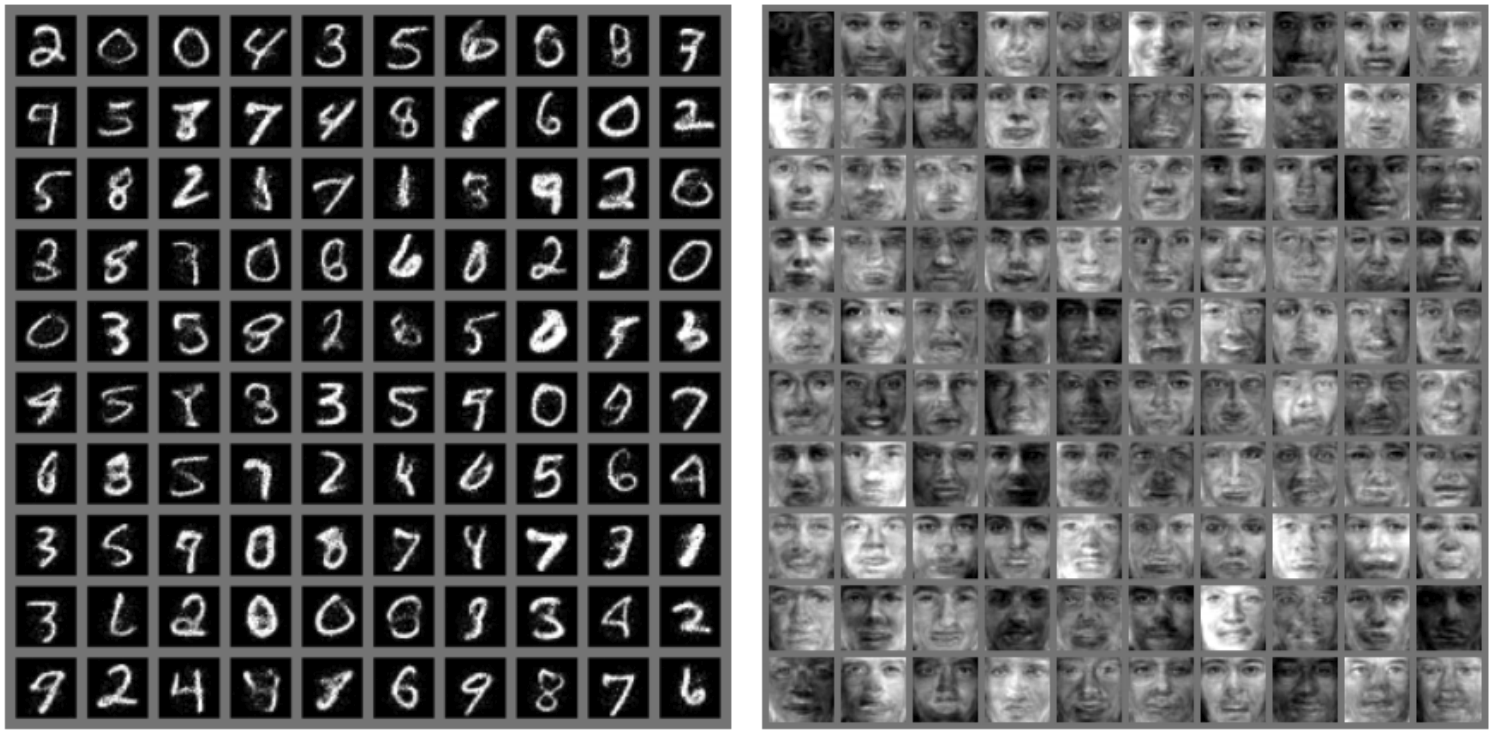
NICE 모델로 MNIST와 TFD 데이터셋을 각각 학습하고 데이터를 생성한 결과는 위와 같다. 모델의 단순함에 비해 꽤 괜찮은 성능을 보이는 것을 알 수 있다.
Real-NVP
Real-NVP는 NICE를 확장한 모델로, NICE가 $m_{\theta}$를 이용해 shift만을 한 것과 달리 Real-NVP에서는 shift와 scale를 모두 수행한다.
Forward mapping $\mathbf{z} \mapsto \mathbf{x}$는 아래와 같이 정의된다.
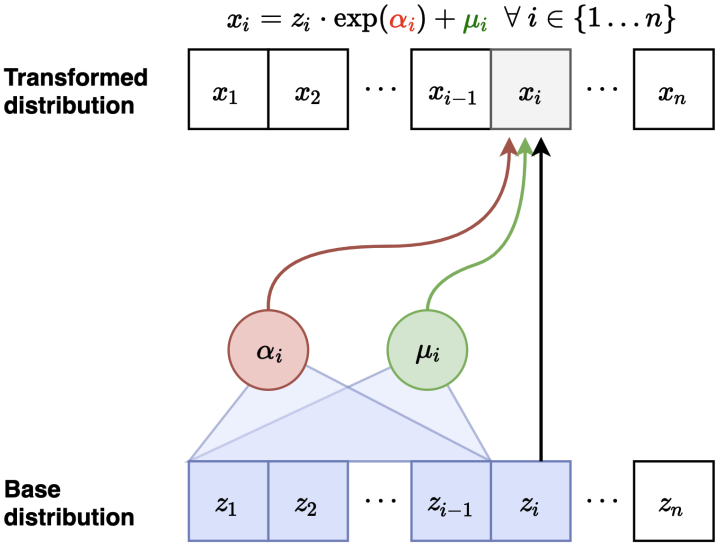
$\begin{gather} \mathbf{x}_{1:d} = \mathbf{z}_{1:d} \\ \mathbf{x}_{d+1:n} = \mathbf{z}_{d+1:n} \odot \exp\big( \alpha_{\theta}(\mathbf{z}_{1:d}) \big) + \mu_{\theta}(\mathbf{z}_{1:d}) \end{gather}$
첫 그룹은 NICE와 마찬가지로 identity mapping이고, 두 번째 그룹은 $\mu_{\theta}$로 shift, $\exp\big( \alpha_{\theta}(\mathbf{z}_{1:d}) \big)$로 element-wise scaling을 한다. $\alpha_{\theta}$와 $\mu_{\theta}$는 뉴럴 네트워크이고, scale을 항상 양수로 만들기 위해 exponential을 취한다. 각 layer에서 $\alpha_{\theta}$와 $\mu_{\theta}$의 파라미터 $\theta$는 모두 다르다.
Inverse mapping $\mathbf{x} \mapsto \mathbf{z}$는 직관적으로 아래와 같이 계산할 수 있다.
$\begin{gather} \mathbf{z}_{1:d} = \mathbf{x}_{1:d} \\ \mathbf{z}_{d+1:n} = \big( \mathbf{x}_{d+1:n} - \mu_{\theta}(\mathbf{x}_{1:d}) \big) \odot \big( \exp(-\alpha_{\theta}(\mathbf{x}_{1:d})) \big) \end{gather}$
Forward mapping에 대한 jacobian은 아래와 같이 구할 수 있다.
$J = \cfrac{\partial \mathbf{x}}{\partial \mathbf{z}} = \begin{pmatrix} I_d & 0 \\ \cfrac{\partial \mathbf{x}_{d+1:n}}{\partial \mathbf{z}_{1:d}} & \text{diag} \big( \exp(\alpha_{\theta}(\mathbf{z}_{1:d})) \big) \end{pmatrix}$
Scaling factor로 인하여 identity 대신 diagonal 항이 존재하는 것을 알 수 있다.
따라서 이 jacobian의 determinant는 아래와 같다.
$\det(J) = \prod\limits_{i=d+1}^{n} \exp(\alpha_{\theta}(\mathbf{z}_{1:d})_i) = \exp \left( \sum\limits_{i=d+1}^{n} \alpha_{\theta}(\mathbf{z}_{1:d})_i \right)$
Scaling factor로 인하여 이 layer들은 non-volume preserving transformation이라고도 불리고, Real-NVP는 NICE보다 훨씬 flexible한 모델이 된다.
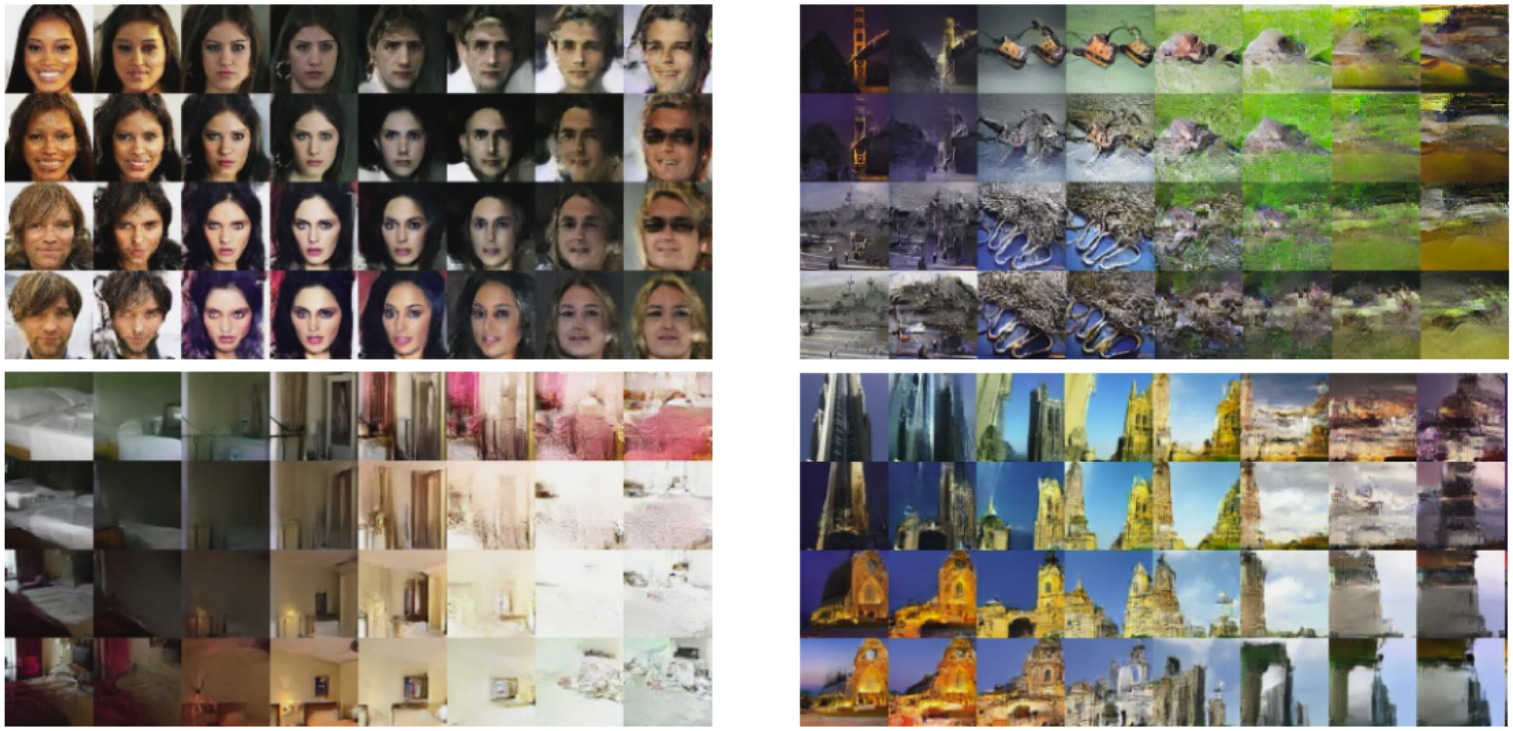
Real-NVP 모델의 결과는 위와 같다. Latent vector를 interpolate하여 두 이미지의 중간에 해당하는 결과를 생성할 수 있다는 것도 확인할 수 있다.
Masked Autoregressive Flow (MAF)
$\mathbf{x}$가 continuous variable일 때 autoregressive model 또한 flow model의 관점으로 생각할 수 있다.
$p(\mathbf{x}) = \prod\limits_{i=1}^{n} p(x_i \mid \mathbf{x}_{\lt i})$
Autoregressive 모델의 기본적인 수식은 위와 같다. 이때 각 조건부 확률 $p(x_i \mid \mathbf{x}_{\lt i})$는 가우시안 분포 $\mathcal{N} \big( \mu_i(x_1, \dots, x_{i-1}), \exp (\alpha_i(x_1, \dots, x_{i-1}))^2 \big)$ 를 따른다고 하자. $\mu_i$와 $\alpha_i$는 뉴럴 네트워크이다.
우선 데이터 생성, 즉 forward mapping을 살펴보자.
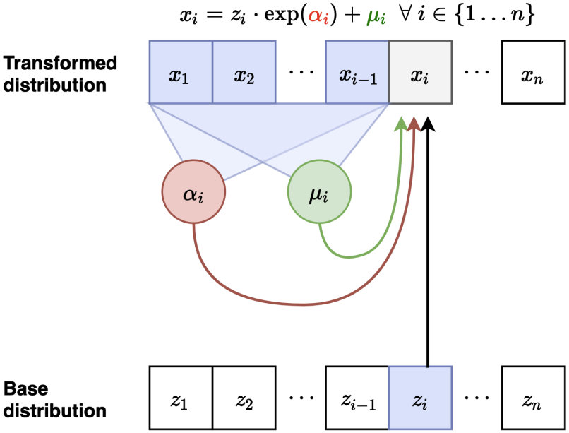
일반적인 autoregressive model과 같이 $x_1$부터 시작해서 순서대로 데이터를 샘플링하게 된다. 이때 reparametrization trick을 포함하여 식을 세우면 아래와 같다.
- $z_1 \sim \mathcal{N}(0, 1)$을 샘플링하고 $x_1 = \exp(\alpha_1)z_1 + \mu_1$을 얻는다.
- $z_2 \sim \mathcal{N}(0, 1)$을 샘플링하고 $\mu_2(x_1), \alpha_2(x_1)$을 계산한다. $x_2 = \exp(\alpha_2)z_2 + \mu_2$을 얻는다.
- $z_3 \sim \mathcal{N}(0, 1)$을 샘플링하고 $\mu_3(x_2), \alpha_3(x_2)$을 계산한다. $x_3 = \exp(\alpha_3)z_3 + \mu_3$을 얻는다.
- 위 과정을 반복한다.
Real-NVP 모델과 식의 형태가 유사함을 볼 수 있다.
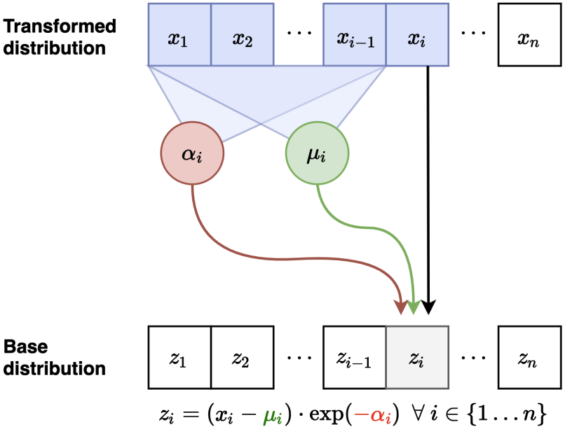
Inverse mapping 시에는 모든 $\mu_i$와 $\alpha_i$를 한번에 계산할 수 있다. 모든 $x_i$가 주어져 있기 때문이다. 이를 이용해 모든 $u_i$를 역으로 한번에 계산할 수 있고, likelihood를 빠르게 계산할 수 있다.
Jacobian 또한 triangular matrix가 된다.
이 과정을 하나의 layer로 삼아 여러 layer를 쌓을 수 있다.
Inverse Autoregressive Flow (IAF)
MAF의 단점은 inference에 여전히 변수를 하나씩 샘플링해야 한다는 점이다. 하지만 Flow model의 관점에서는 forward mapping과 inverse mapping이 모두 쉽게 가능하기 때문에 $\mathbf{x}$와 $\mathbf{z}$의 역할을 바꾸는 것으로 이를 해결할 수 있다. 이러한 모델이 바로 IAF이다.
IAF는 모든 $x_i$를 한번에 생성할 수 있고 생성한 데이터 $\mathbf{x}$에 대해 likelihood도 한번에 구할 수 있다. $\mathbf{z}$를 이미 알고 있기 때문이다. 반대로 학습 시에는 $z_i$를 하나씩 생성해야 하기 때문에 training 시 likelihood를 구하는 것은 느리다.
Parallel Wavenet
Parallel wavenet은 MAF와 IAF의 장점을 합친 모델로, 잘 학습된 MAF를 IAF로 distill하는 방식이다. Distillation에 사용하는 수식은 아래와 같다.
$D_{KL}(s, t) = \mathbb{E}_{x \sim s} \big[ \log s(\mathbf{x}) - \log t(\mathbf{x}) \big]$
$s(\mathbf{x})$는 student model인 IAF에서의 likelihood, $t(\mathbf{x})$는 teacher model인 MAF에서의 likelihood이다.
먼저 IAF에서 샘플 $\mathbf{x}$를 하나 생성한다. IAF는 자신이 생성한 데이터에 대해서는 likelihood $s(\mathbf{x})$를 빠르게 구할 수 있다. 또한 MAF는 likelihood 연산 자체를 빠르게 할 수 있으므로 $t(\mathbf{x})$도 빠르게 구할 수 있다.
이 KL divergence를 최소화함으로써 잘 학습된 MAF의 정보를 쉽게 IAF로 distill할 수 있다. 이 방식을 이용한 Parallel wavenet은 기존 autoregressive model에 비해 1000배 빠르다고 한다.
MintNet
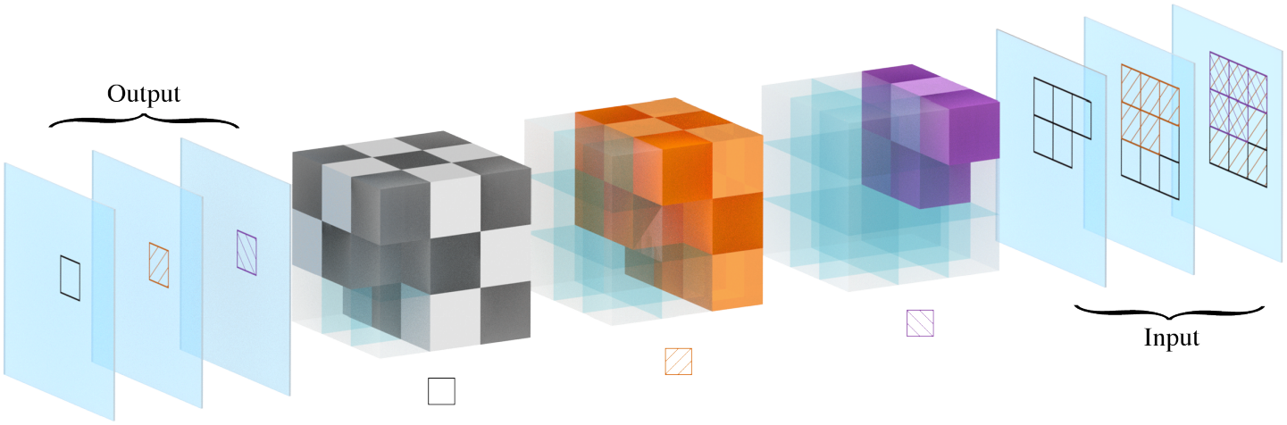
PixelCNN과 같이 CNN도 autoregressive model처럼 생각할 수 있는데, 이를 flow model에 적용한 것이 MintNet이다. 위 그림과 같이 kernel을 잘 masking하여 CNN을 invertible하게 만들 수 있다.
Gaussianization Flows
Gaussianization flows 모델은 flow model의 학습을 다른 방식으로 생각한다. 기존에는 flow model로부터 생성한 데이터의 distribution이 실제 data distribution과 같아지도록 학습한다고 생각한다면, Gaussian flows에서는 데이터들을 inverse mapping을 통해 변환했을 때 prior인 Gaussian distribution과 같아지도록 학습한다고 생각한다.
그 방법을 inverse CDF trick이라고 하는데, 실제 data distribution의 CDF를 이용하여 데이터를 가우시안 분포로 변환하는 방법이다.
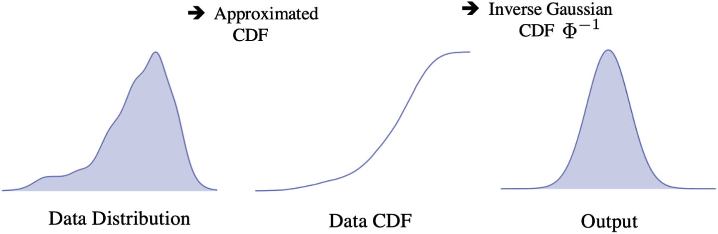
우선 실제 data distribution의 CDF를 구한다. 그러면 특정 데이터 $\mathbf{x}$에 대한 누적 확률값을 0부터 1 사이의 값으로 얻을 수 있다. 이 값을 가우시안 분포의 inverse CDF에 입력시키면 동일한 누적 확률값을 가지는 가우시안 분포의 한 점을 얻을 수 있다.
이러한 layer를 여러 개 쌓음으로써 주어진 데이터셋을 점점 더 가우시안 분포에 가깝도록 transform시킬 수 있다.
Summary
Normalizing flow model을 요약하면 아래와 같다.
- Normalizing flow model은 change of variables 공식을 이용해 단순한 분포를 더욱 복잡한 분포로 변환시킨다.
- Transformation의 jacobian을 효율적으로 구할 수 있어야 한다.
- Forward mapping과 inverse mapping 사이에 computational tradeoff가 존재한다.